Pine Island Glacier Sensitivity Study
Goals
This example is adapted from the results presented in [Seroussi2014]. We model the impact of different external forcings on the dynamic evolution of Pine Island Glacier. The main objectives are to:
- Run transient simulations (10 years) of a real glacier
- Change external forcings
- Compare the impact of changes on glacier dynamics and volume
Files needed to run this tutorial are located in <ISSM_DIR>/examples/PigSensitivity/. This tutorial relies on experience gained from completing the Pine Island Glacier and Greenland Ice Sheet modeling tutorials, so make sure to complete them first.
Evolution over 10 years
We first run a simulation of Pine Island Glacier over a 10 year period, starting from the Pig tutorial.
In the runme.m file, several parameters are adjusted before running the transient model. Open runme.m and make sure that the variable steps, at the top of the file, is set to steps = [1]. In the code, you will see that in step 1 the following actions are implemented:
- Load model from the
Pigtutorial - Apply some basal melting rate
- On grounded ice:
md.basalforcings.groundedice_melting_rate - On floating ice:
md.basalforcings.floatingice_melting_rate
- On grounded ice:
- Specify time step length and run duration in
md.timestepping - Disable inverse method in
md.inversion.iscontrol = 0 - Indicate what components of the transient to activate
md.transient.ismasstransportmd.transient.isstressbalancemd.transient.isthermalmd.transient.isgroundinglinemd.transient.ismovingfront
- Request additional outputs
- Solve transient solution
Execute runme to perform step 1. The following figure shows the evolution of the ice velocity and grounding line positions at the beginning and at the end of the simulation:

Increased basal melting rate
In this second step, we increase the basal melting rate under the floating portion of the domain from 25 to 60 m/yr. The other parameters remain the same as in the previous step.
Open runme.m and change the step at the top of the file to step = 2, then run the simulation. The following figure shows the evolution of ice velocity and grounding line evolution for the increased melting scenario:

Retreat of ice front position
In this third step, we would like to test the sensitivity of Pig to calving events and retreat the position of the ice front. We first need to create a new contour of the region to be removed from the domain. Use exptool to create a new RetreatFront.exp contour that include the portion of floating ice that should calve off.
Then extract the domain from the initial model, excluding the RetreatFront.exp area using the extrude routine:
>> md2 = modelextract(md, ~RetreatFront.exp)
As this operation changes the model domain, some parameters and boundary conditions have the be adjusted or redefined.
The boundary conditions are reset with SetMarineIceSheetBC and the model can then be solved.
Open runme.m and change the step at the top of the file to step = 3, then run the simulation. The following figure shows the evolution of ice velocity and grounding line evolution with the new ice front:
Change in surface mass balance
In this last step, we change the surface mass balance, while the other parameters remain similar to the previous simulations.
Open runme.m and implement the changes needed to investigate the impact of the surface mass balance, similar to what was done with the other external forcings in the previous steps. These changes are:
- Load model from the
Pigtutorial - Change the surface mass balance
- Verify the ocean-induced melting rate
- On grounded ice:
md.basalforcings.groundedice_melting_rate - On floating ice:
md.basalforcings.floatingice_melting_rate
- On grounded ice:
- Specify time step length and run duration in
md.timestepping - Disable inverse method in
md.inversion.iscontrol - Indicate what components of the transient to activate
md.transient.ismasstransportmd.transient.isstressbalancemd.transient.isthermalmd.transient.isgroundinglinemd.transient.ismovingfront
- Request additional outputs
- Solve transient solution
Don’t forget to change step at the top of the runme.m.
Below is the solution to make this change:
if step == 4
	%Load model
	md = loadmodel('./Models/PIG_Transient');

	%Change external forcing basal melting rate and surface mass balance)
	md.basalforcings.groundedice_melting_rate = zeros(md.mesh.numberofvertices, 1);
	md.basalforcings.floatingice_melting_rate = 25 * ones(md.mesh.numberofvertices, 1);
	md.smb.mass_balance = 2 * md.smb.mass_balance;

	%Define time steps and time span of the simulation
	md.timestepping.time_step = 0.1;
	md.timestepping.final_time = 10;

	%Request additional outputs
	md.transient.requested_outputs = {'default', 'IceVolume', 'IceVolumeAboveFloatation'};

	%Solve
	md = solve(md, 'Transient');

	%Plot
	plotmodel(md, 'data', md.results.TransientSolution(1).Vel, ...
		'title#1', 'Velocity t=0 years (m/yr)', ...
		'data', md.results.TransientSolution(end).Vel, ...
		'title#2', 'Velocity t=10 years (m/yr)', ...
		'data', md.results.TransientSolution(1).MaskOceanLevelset, ...
		'title#3', 'Floating ice t=0 years', ...
		'data', md.results.TransientSolution(end).MaskOceanLevelset, ...
		'title#4', 'Floating ice t=10 years', ...
		'caxis#1', ([0 4500]), 'caxis#2', ([0 4500]), ...
		'caxis#3', ([-1, 1]), 'caxis#4', ([-1, 1]));

	%Save model
	save ./Models/PIG_SMB md;
end
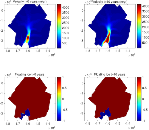
Here is an example of velocity change and grounding line evolution when the surface mass balance is doubled:

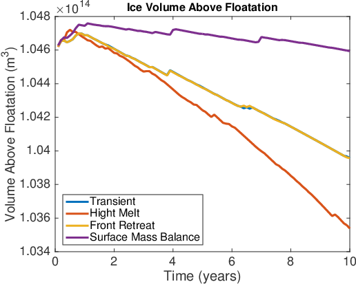
Evolution of the ice volume above flotation
In the previous steps, we investigated the impact of changes in external forcings on ice flow dynamics (grounding line evolution and glacier acceleration). We can also see how these changes impact the glacier volume and its contribution to sea level rise. To do so, we use the additional output IceVolumeAboveFloatation requested in the transient simulation. The following figure shows the evolution of the volume (in Gt/yr) above flotation for the four scenarios performed previously:
References
- H. Seroussi, M. Morlighem, E. Rignot, J. Mouginot, E. Larour, M. P. Schodlok, and A. Khazendar. Sensitivity of the dynamics of Pine Island Glacier, West Antarctica, to climate forcing for the next 50 years. Cryosphere, 8(5):1699-1710, 2014.