Mesh Adaptation

Goals

In this tutorial, we show how to use the different meshers of ISSM:

• Learn how to use the different meshers of ISSM:
  • squaremesh for square domains (ISMIP)
  • roundmesh for round domain (EISMINT)
  • triangle (from J. Shewchuk)
  • bamg (adapted from F. Hecht)
• Use anisotropic mesh adaptation to optimize the mesh resolution spatially Go to <ISSM_DIR>/examples/Mesh/ to do this tutorial.

Squaremesh

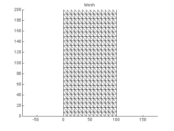
squaremesh generates structured uniform meshes for rectangular domains.

Usage

>> md = model;
>> md = squaremesh(md, 100, 200, 15, 25);

squaremesh takes the following arguments:

1. model
2. x-length (meters)
3. y-length (meters)
4. number of nodes along the x axis
5. number of nodes along the y axis

Example

The previous command creates the mesh shown below:

>> plotmodel(md, 'data', 'mesh');

Roundmesh

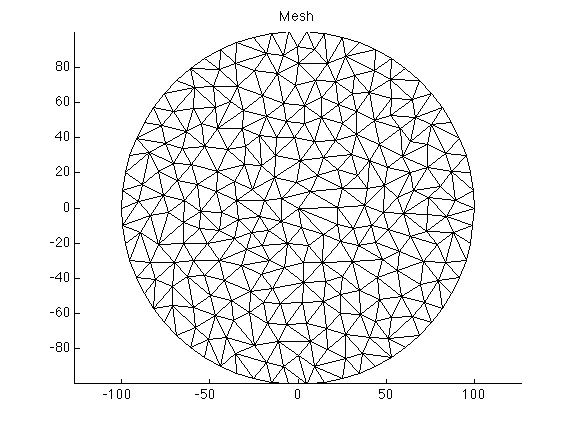
roundmesh generates unstructured uniform meshes for circular domains.

Usage

>> md = roundmesh(model, 100, 10);

roundmesh takes the following arguments:

1. model
2. radius (meters)
3. element size (meters)

Example

The previous command creates the mesh shown below:

>> plotmodel(md, 'data', 'mesh');

Triangle

triangle is a very fast algorithm for mesh generation. Developed by J Shewchuk, it generates unstructured triangular meshes.

Usage

>> md = triangle(model, 'Square.exp', .2);

triangle takes the following arguments:

1. model
2. ARGUS file of the domain outline (.exp extension, see the ‘Capabilities’ → ‘Mesh Generation’ page for more details)
3. average element size (meters) The previous command creates the following mesh:

   >> plotmodel(md, 'data', 'mesh');
   

You can change the resolution from 0.2 to 0.05 to get a higher resolution.

Bamg

BAMG stands for Bidimensional Anisotropic Mesh Generator. It was released in 2006 after more than 10 years of development by Frederic Hecht. It is now part of FreeFEM++. The algorithm that is available in ISSM is inspired by this software, but has been rewritten entirely.

Usage

>> md = bamg(model, ...);

bamg takes as it’s first argument a model, and then pairs of options

1. model
2. pairs of options (type help bamg to get a full list of options)

Uniform mesh

To create a non-uniform mesh, use the following options:

1. 'domain' followed by the domain name
2. 'hmax' followed by the size (meters) of each triangle

   >> md = bamg(model, 'domain', 'Square.exp', 'hmax', .05);
   

   The previous command will create the following mesh (use plotmodel(md, 'data', 'mesh') to visualize the mesh):

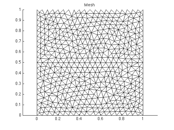
Note that the nodes are not as randomly distributed as triangle. The strength of BAMG is not for uniform meshes but for automatic mesh adaptation based on a metric.

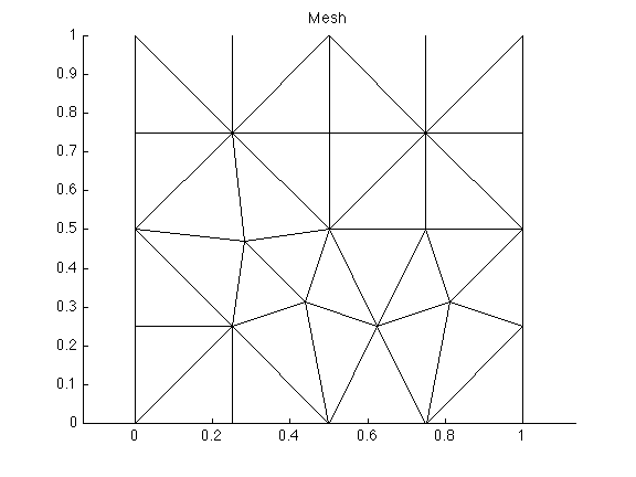
Non-Uniform mesh

To create a non-uniform mesh, use the following options:

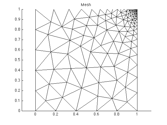
1. 'domain' followed by the domain name
2. 'hvertices' followed by the element size for each vertex of the domain outline In our example, Square.exp has 4 vertices. If we want a resolution of 0.2, except in the vicinity of the third node, we use the following commands:

   >> md = model;
   >> hvertices = [0.2; 0.2; 0.005; 0.2];
   >> md = bamg(md, 'domain', 'Square.exp', 'hvertices', hvertices);
   

   Use the plotmodel(md, 'data', 'mesh') command to visualize the newly defined mesh:

Mesh adaptation

We can use observations to generate a mesh that is adapted to the solution we are trying to model. Given a solution field, bamg will calculate a metric based on the field’s Hessian matrix (second derivative) to generate an anisotropic mesh that minimize the interpolation error (assuming that linear finite elements are used).

For a first example, we are going to use the observations given by the function shock.m. It generates a discontinuity that requires the mesh to be highly refined along a circle.

First, we generate a simple uniform mesh. We interpolate the observations on the vertices of this mesh:

>> md = bamg(model, 'domain', 'Square.exp', 'hmax', .05);
>> vel = shock(md.mesh.x, md.mesh.y);
>> plotmodel(md, 'data', vel, 'edgecolor', 'w');

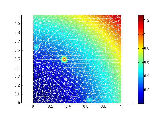
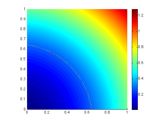
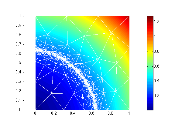
With a simple uniform mesh, the discontinuity is not captured. It is best to start with a finer mesh, which captures the discontinuity rather well, and interpolate the observations on this finer mesh to adapt the mesh anisotropically.

>> md = bamg(model, 'domain', 'Square.exp', 'hmax', .005);
>> vel = shock(md.mesh.x, md.mesh.y);

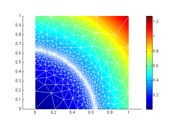
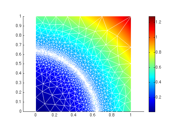
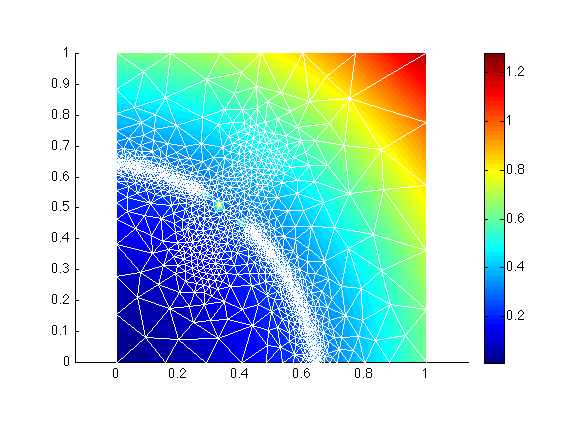
Now, we call bamg a second time to adapt the mesh according the vel. We do not reinitialize md and call bamg again without specifying the 'domain', as a first mesh already exists in the model. We provide the following options:

1. 'field' followed by vel, the field we want to adapt the mesh to
2. 'err' the allowed interpolation error (Here, the field must be captured within 0.05)
3. 'hmin' minimum edge length
4. 'hmax' maximum edge length

   >> md = bamg(md, 'field', vel, 'err', 0.05, 'hmin', 0.005, 'hmax', 0.3);
   >> vel = shock(md.mesh.x, md.mesh.y);
   >> plotmodel(md, 'data', vel, 'edgecolor', 'w');
   

You can change the option 'err' to 0.03, to see the effect of 'err'. The ratio between two consecutive edges can be controlled by the option 'gradation'.

>> md = bamg(model, 'domain', 'Square.exp', 'hmax', .005);
>> vel = shock(md.mesh.x, md.mesh.y);
>> md = bamg(md, 'field', vel, 'err', 0.03, 'hmin', 0.005, 'hmax', 0.3, 'gradation', 3);
>> vel = shock(md.mesh.x, md.mesh.y);
>> plotmodel(md, 'data', vel, 'edgecolor', 'w');

We can also force the triangles to be equilateral by using the 'anisomax' option, which specifies the maximum level of anisotropy (between 0 and 1, 1 being fully isotropic).

>> md = bamg(model, 'domain', 'Square.exp', 'hmax', .005);
>> vel = shock(md.mesh.x, md.mesh.y);
>> md = bamg(md, 'field', vel, 'err', 0.03, 'hmin', 0.005, 'hmax', 0.3, 'gradation', 1.3, 'anisomax', 1);
>> vel = shock(md.mesh.x, md.mesh.y);
>> plotmodel(md, 'data', vel, 'edgecolor', 'w');

You can also try to refine a mesh using the function circles.m, which is provided in the same directory.

Mesh refinement in a specific region

It is sometimes necessary to specify a mesh resolution for an area of interest. We will use the same example as before. The first step consists of creating an ARGUS file that defines the region where we want to refine the mesh.

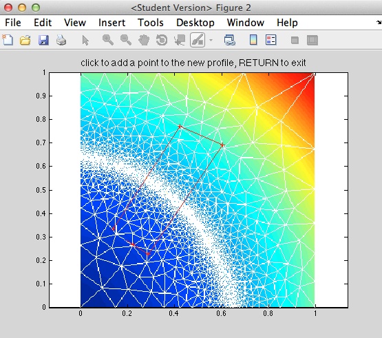
We first plot vel and we call the function exptool to create a file refinement.exp that defines this region. Select add a contour (closed). Draw a contour over a given region, hit enter when you are done, and then select quit. You should now see the refinement.exp file in the current directory.

>> plotmodel(md, 'data', vel, 'edgecolor', 'w');
>> exptool('refinement.exp')

Now, we are going to create a vector that specifies, for each vertex of the existing mesh, the resolution of the adapted mesh. We use NaN for the vertices we do not want to change. So in this example, this will be a vector of NaN, except for the vertices in refinement.exp, where we want a resolution of 0.02:

>> h = NaN * ones(md.mesh.numberofvertices, 1);
>> in = ContourToNodes(md.mesh.x, md.mesh.y, 'refinement.exp', 1);
>> h(find(in)) = 0.02;
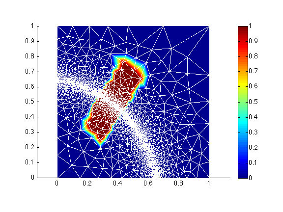
>> plotmodel(md, 'data', in, 'edgecolor', 'w');

You will see that all the vertices that are in refinement.exp have a value of 1 (they are inside the contour), and the others are 0.

Now, we call bamg a third time, with the specified resolution for the vertices that are in refinement.exp:

>> vel = shock(md.mesh.x, md.mesh.y);
>> md = bamg(md, 'field', vel, 'err', 0.03, 'hmin', 0.005, 'hmax', 0.3, 'hVertices', h);
>> vel = shock(md.mesh.x, md.mesh.y);
>> plotmodel(md, 'data', vel, 'edgecolor', 'w');

Another example

If you would like to try another example, you can use the function circles.m instead of shock.m. It is also a 1x1 square but with a pattern that includes five circles.