Subglacial Hydrology of Helheim Glacier (SHAKTI)
Goals
- Use SHAKTI model to simulate subglacial hydrology of Helheim Glacier in southeast Greenland
- Follow an example of how to set up a SHAKTI hydrology simulation on a real-world glacier
- Learn how to run a two-way coupled hydrology—velocity model with SHAKTI-ISSM
- Run a coupled SHAKTI-ISSM simulation of winter base-state hydrology
- Run a coupled SHAKTI-ISSM simulation with transient seasonal meltwater inputs (distributed and point inputs)
Introduction
In this example, the main goal is to set up a subglacial hydrology simulation using the SHAKTI model, coupled with ice velocity on a real Greenland outlet glacier. In order to build an operational simulation of Helheim Glacier as an example, we will follow these steps:
- Load your Helheim Glacier model created in the ‘Modeling Helheim Glacier’ tutorial
- Set the hydrology model to SHAKTI and set up friction coupling
- Set SHAKTI-specific hydrology parameters
- Run a transient two-way coupled simulation with zero meltwater input to generate the winter base state drainage system
- Set up and run two-way coupled seasonal simulations with prescribed distributed meltwater input and point meltwater inputs
Files needed for this tutorial can be found in <ISSM_DIR>/examples/HelheimSHAKTI/. This tutorial begins from a model of Helheim Glacier generated in the ‘Modeling Helheim Glacier’ tutorial.
Load model
The first step in the runme.m file is to load the model of Helheim Glacier created in the previous tutorial. We turn off the inversion now.
Set up SHAKTI subglacial hydrology model
In the runme.m file, we set the hydrology model to SHAKTI: md.hydrology = hydrologyshakti();
Next, we initialize the SHAKTI-specific hydrological parameters:
- Distributed meltwater input (“englacial input”) (m yr-1)
- Point meltwater input (“moulin input”) (m3 s-1)
- Initial hydraulic head (m)
- Initial subglacial gap height (m)
- Typical bed bump height and spacing (m)
- Initial Reynolds number
- Boundary conditions (prescribed head for thin ice and ice-free elements)
Define coupling and friction
We turn on the coupling between SHAKTI and ISSM through md.transient and md.friction.coupling. This tutorial uses the Budd-type sliding law.
- To turn on SHAKTI, set
md.transient.ishydrology = 1. - To solve for stress balance in the transient simulation, set
md.transient.isstressbalance = 1andmd.friction.coupling = 4. - To run stand-alone SHAKTI without evolving velocity, set
md.transient.isstressbalance = 0.
Run a winter simulation
The final step before running is to define the time step and final time of the simulation. Note that the time step and final time set in years, so make sure to convert appropriately. Small time steps on the order of 1 hour are typically functional for SHAKTI, but feel free to experiment with this.
The model will take a while to run, exactly how long will vary depending on your final time, time step, how many processors you are using, and mesh resolution. If you are running a long simulation, you might not want to save model output at every time step and can reduce the output file size through md.settings.output_frequency (for example, with a time step of 1 hour, you would set md.settings.output_frequency = 24; to save output once every day).
The model you have set up currently specifies zero meltwater inputs (md.hydrology.englacial_input and md.hydrology.moulin_inputs are both zero everywhere). This represents winter conditions, when all water at the bed is generated via basal melt by geothermal flux, frictional heat from sliding, and turbulent dissipation.
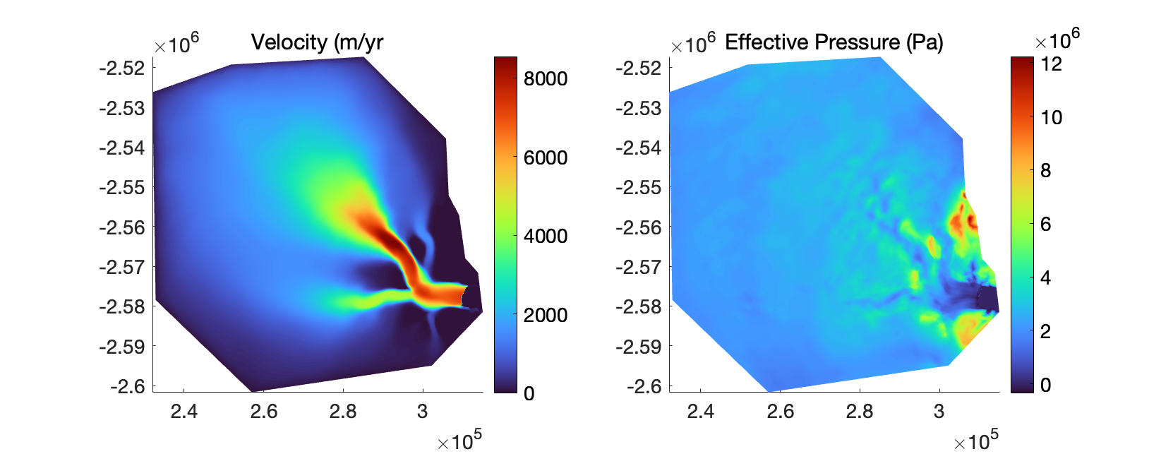
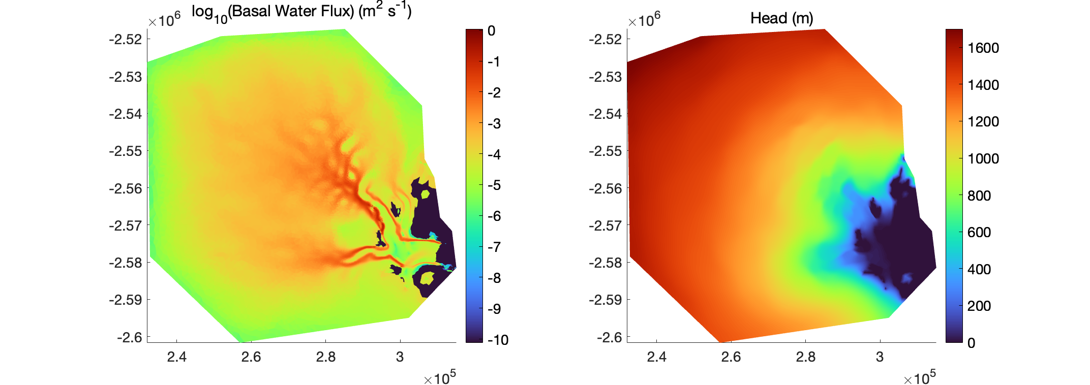
You can examine the output spatially by plotting different quantities. For example, here are plots of velocity, effective pressure, basal water flux, and hydraulic head after 30 days:
plotmodel(md, 'data', md.results.TransientSolution(end).Vel, 'title', 'Velocity (m/yr)', ...
	'data', md.results.TransientSolution(end).EffectivePressure, 'title', 'Effective Pressure (Pa)')
plotmodel(md, 'data', log10(md.results.TransientSolution(end).HydrologyBasalFlux), 'title', 'log_{10}(Basal Water Flux) (m^2 s^{-1})', ...
	'data', md.results.TransientSolution(end).HydrologyHead, 'title', 'Head (m)')
If you are interested in a steady state, check convergence to a steady winter state by comparing md.results.TransientSolution(end).Vel and md.results.TransientSolution(end).EffectivePressure with the previous time step. You will probably need to run for a year or two for the system to fully equilibrate.
Continuing a simulation
You may find it helpful to continue a simulation from the end state of a previous simulation. This can be useful for running long simulations in segments or exploring different forcing from a common initialized state. Use the script below to continue a previous simulation, which sets the relevant initial parameters accordingly:
% runme script to continue a coupled SHAKTI-ISSM simulation, continuing from
% end state of a previous simulation

clear all; close all

% Load the model you want to begin from
load Models/your_shaktiissm_model_name.mat

% Starting conditions from end of previous simulation
md.hydrology.head = md.results.TransientSolution(end).HydrologyHead;
md.hydrology.gap_height = md.results.TransientSolution(end).HydrologyGapHeight;
md.hydrology.reynolds = md.results.TransientSolution(end).HydrologyBasalFlux ./ 1.787e-6;
md.hydrology.reynolds(md.hydrology.reynolds == 0) = 1;

md.initialization.vx = md.results.TransientSolution(end).Vx;
md.initialization.vy = md.results.TransientSolution(end).Vy;
md.initialization.vel = md.results.TransientSolution(end).Vel;

% Time-stepping
md.timestepping.time_step = 3600 / md.constants.yts; % Time step (in years)
md.timestepping.final_time = 365 / 365;
md.settings.output_frequency = 24;

md.cluster = generic('np', 8);
md.verbose.solution = 1;
md = solve(md, 'Transient');
Seasonal meltwater inputs
Meltwater inputs can be added through two options:
- Distributed meltwater input (e.g. for highly crevassed regions):
md.hydrology.englacial_input(units of m yr-1) - Point inputs to represent discrete crevasses or moulins:
md.hydrology.moulin_input(units of m3 s-1)
Both types of meltwater input are spatially variable and can be prescribed as either constant in time (size(md.mesh.numberofvertices, 1)) or time-varying (size(md.mesh.numberofvertices + 1, length(timevec))). The sample code below includes example syntax for setting these meltwater inputs. Get creative and experiment with different combinations!
% Time-stepping
md.timestepping.time_step = 3600 / md.constants.yts; % Time step (in years)
md.timestepping.final_time = 365 / 365;
timevec = 0:md.timestepping.time_step:md.timestepping.final_time;
md.settings.output_frequency = 24;

% To prescribe distributed meltwater inputs:
% Steady distributed meltwater inputs:
md.hydrology.englacial_input = zeros(md.mesh.numberofvertices, 1);
md.hydrology.englacial_input(:) = **set values here, can vary spatially**;

% Time-varying distributed meltwater inputs:
% Initialize the matrix as zeros
md.hydrology.englacial_input = zeros(md.mesh.numberofvertices + 1, length(timevec));
% Set the final column to be a time index
md.hydrology.englacial_input(end, :) = timevec;
% Example: low-elevation distributed meltwater inputs
le = find(md.geometry.surface <= 900); % Find low-elevation vertices below 900 m
for nv=1:length(le)
md.hydrology.englacial_input(le(nv), :) = <<your data or function here>>;
end

% To prescribe point meltwater inputs:
% Example: Steady input into firn aquifer crevasse drainage points
% Find high-elevation crevasse input points from firn aquifer at 1500 m
he = find(md.geometry.surface >= 1500 & md.geometry.surface <= 1515);
highieb = 1.5855 / size(he, 1); % Use 50e6 m^3/yr, converted to m^3/s, divided evenly between eligible points
md.hydrology.moulin_input = zeros(md.mesh.numberofvertices, 1);
md.hydrology.moulin_input(he) = highieb;

% For time-varying point inputs:
md.hydrology.moulin_input = zeros(md.mesh.numberofvertices + 1, length(timevec));
md.hydrology.moulin_input(end, :) = timevec;
md.hydrology.moulin_input(1:end-1, :) = **set values here, can vary spatially and temporally**
Resources
For more details about the SHAKTI model and applications to Helheim Glacier, please see the following references: [Sommers2018,Sommers2023,Sommers2024].
References
-
A. Sommers, H. Rajaram, and M. Morlighem. SHAKTI: Subglacial Hydrology and Kinetic, Transient Interactions v1.0. Geosci. Model Dev., 11(7):2955-2974, 2018.
-
A. N. Sommers, C. R. Meyer, K. Poinar, J. Mejia, M. Morlighem, H. Rajaram, K. L. P. Warburton, and W. Chu. Velocity of Greenland’s Helheim Glacier Controlled Both by Terminus Effects and Subglacial Hydrology With Distinct Realms of Influence. Geophys. Res. Lett., 51(15):e2024GL109168, 2024.
-
Aleah Sommers, Colin Meyer, Mathieu Morlighem, Harihar Rajaram, Kristin Poinar, Winnie Chu, and Jessica Mejia. Subglacial hydrology modeling predicts high winter water pressure and spatially variable transmissivity at Helheim Glacier, Greenland. J. Glaciol., page 1–13, 2023.