Basal Melt
Table of Contents
- Default/prescribed melt rate (basalforcings)
- Beckmann and Goosse (2003) parameterization (basalforcingsbeckmanngoosse)
- ISMIP6 quadratic melt parameterization (basalforcingsismip6)
- PICO and PICOP (basalforcingspico)
- Example: the Amundsen Sea
- References
Basal melt controls the mass balance of grounded ice in contact with subglacial water and, more importantly, of floating ice shelves in contact with the ocean. ISSM offers several parameterizations for it, ranging from a simple prescribed rate to physically based schemes that compute melt from far-field ocean temperature and salinity. The parameterization is selected by assigning the corresponding class to md.basalforcings.
Default/prescribed melt rate (basalforcings)
The simplest option prescribes the basal melting rate directly, uniformly or spatially/temporally varying, on grounded and floating ice separately:
>> md.basalforcings = basalforcings();
md.basalforcings.groundedice_melting_rate: basal melting rate applied to grounded ice (positive if melting) [m/yr]md.basalforcings.floatingice_melting_rate: basal melting rate applied to floating ice (positive if melting) [m/yr]md.basalforcings.perturbation_melting_rate: (optional) perturbation in basal melting rate under floating ice [m/yr]md.basalforcings.geothermalflux: geothermal heat flux [\(W/m^2\)]
Beckmann and Goosse (2003) parameterization (basalforcingsbeckmanngoosse)
This parameterization, from [Beckmann2003], relates the melt rate under floating ice to the difference between the far-field ocean temperature \(T_{oc}\) and the local freezing point \(T_f\) at the depth of the ice-shelf base:
\[m = e_0 \frac{\rho_w c_{p,w} \gamma_T}{\rho_i L}\left(T_{oc} - T_f\right)\]where \(\rho_w\) and \(\rho_i\) are the ocean and ice densities, \(c_{p,w}\) is the specific heat capacity of the ocean mixed layer, \(\gamma_T\) is a turbulent heat exchange velocity, \(L\) is the latent heat of fusion, and \(e_0\) (meltrate_factor) is a tunable calibration factor. The local freezing point is estimated from a linear equation of state:
where \(S\) is the local ocean salinity and \(z_b\) is the ice-shelf draft elevation.
>> md.basalforcings = basalforcingsbeckmanngoosse();
md.basalforcings.groundedice_melting_rate: basal melting rate applied to grounded ice (positive if melting) [m/yr]md.basalforcings.geothermalflux: geothermal heat flux [\(W/m^2\)]md.basalforcings.meltrate_factor: melt-rate calibration factor \(e_0\) (default: 0.5)md.basalforcings.isthermalforcing: whether to useocean_tempandocean_salinity(0, default) orocean_thermalforcing(1)md.basalforcings.ocean_temp: far-field ocean temperature [℃] (used ifisthermalforcingis 0)md.basalforcings.ocean_salinity: far-field ocean salinity [psu] (used ifisthermalforcingis 0)md.basalforcings.ocean_thermalforcing: ocean thermal forcing, \(T_{oc} - T_f\) [K] (used ifisthermalforcingis 1)
ISMIP6 quadratic melt parameterization (basalforcingsismip6)
This parameterization, from [Jourdain2020], was designed for the ISMIP6 Antarctic ice sheet projections. Melt is a quadratic function of the thermal forcing \(TF\) (the difference between the ocean temperature and the local freezing point at depth), evaluated either locally:
\[m = \gamma_0 \left(\frac{\rho_{sw} c_{p,w}}{\rho_i L}\right)^2 \max\left(TF + \delta T, 0\right)^2\]or non-locally, using the thermal forcing averaged over the whole basin, \(\left<TF\right>\):
\[m = \gamma_0 \left(\frac{\rho_{sw} c_{p,w}}{\rho_i L}\right)^2 \left(TF + \delta T\right)\left(\left<TF\right> + \delta T\right)\]where \(\gamma_0\) is a melt-rate coefficient calibrated against observed melt rates, and \(\delta T\) is a basin-specific ocean temperature correction.
>> md.basalforcings = basalforcingsismip6();
md.basalforcings.num_basins: number of basins the model domain is partitioned into [unitless]md.basalforcings.basin_id: basin number assigned to each node [unitless]md.basalforcings.gamma_0: melt rate coefficient \(\gamma_0\) [m/yr] (default: 14477)md.basalforcings.tf_depths: elevation of the vertical layers in the ocean thermal forcing datasetmd.basalforcings.tf: thermal forcing \(TF\) (ocean temperature minus freezing point) at each of these depths [℃]md.basalforcings.delta_t: ocean temperature correction \(\delta T\) per basin [℃]md.basalforcings.islocal: boolean to use the local (1) or non-local (0, default) version of the parameterizationmd.basalforcings.geothermalflux: geothermal heat flux [\(W/m^2\)]md.basalforcings.groundedice_melting_rate: basal melting rate applied to grounded ice (positive if melting) [m/yr]md.basalforcings.melt_anomaly: floating-ice basal melt anomaly [m/yr]
PICO and PICOP (basalforcingspico)
These parameterizations are described in [Reese2018] and [Pelle2019]. They calculate basal melt rates under ice shelves based only on far field ocean temperature and salinity.
PICO is a box model of ocean circulation under ice shelf cavities. Each ice shelf is divided into a set of boxes, and the temperature (\(T_k\)) and salinity (\(S_k\)) of each box is given by:
\[\begin{array}{l c l} \displaystyle q\left(T_{k-1} - T_k\right) - A_k m_k \frac{\rho_i}{\rho_w} \frac{L}{c_p}& =& 0\\ \\ q\left(S_{k-1} - S_k\right) - A_k m_k S_k & =& 0 \end{array}\]where:
- \(A_k\) is the surface area of box \(k\)
- \(m_k\) is the melt rate in box \(k\)
- \(q = C \left(\rho_0 - \rho_1\right)\) is the strength of the overturning circulation
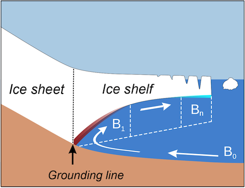
Schematic view of the PICO model (taken from [Reese2018]).
PICOP is described in [Pelle2019]. The idea is to use PICO to calculate the temperature and salinity in each box, but instead of using PICO’s calculated melt, use these quantities to drive a plume model from [Lazeroms2018]:
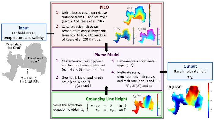
Melt calculation in PICOP, adapted from [Pelle2019]. To activate this melt parameterization, you need to use the class basalforcingspico:
>> md.basalforcings = basalforcingspico();
The parameters relevant to the calculation can be displayed by running:
>> md.basalforcings
md.basalforcings.num_basins: number of basins the model domain is partitioned into [unitless]md.basalforcings.basin_id: basin number assigned to each node [unitless]md.basalforcings.maxboxcount: maximum number of boxes initialized under all ice shelvesmd.basalforcings.overturning_coeff: overturning strength [\(m^3\)/s]md.basalforcings.gamma_T: turbulent temperature exchange velocity [m/s]md.basalforcings.farocean_temperature: depth-averaged ocean temperature in front of the ice shelf for basin i [K]md.basalforcings.farocean_salinity: depth-averaged ocean salinity in front of the ice shelf for basin i [psu]md.basalforcings.isplume: boolean to use buoyant plume melt rate parameterization from Lazeroms et al., 2018 (PICOP, default false)
Example: the Amundsen Sea
To set up a model of the Amundsen Sea using PICOP, we only need one basin:
>> md.basalforcings = basalforcingspico();
>> md.basalforcings.basin_id = ones(md.mesh.numberofelements, 1);
>> md.basalforcings.num_basins = 1;
We generally do not need to have more than 5 boxes per ice shelf:
>> md.basalforcings.maxboxcount = 5;
and finally, we can prescribe the far field ocean properties (they can be time series):
>> md.basalforcings.farocean_temperature = [0.47 + 273.15]; %0.47C converted to K
>> md.basalforcings.farocean_salinity = [34.73]; %PSU
To activate PICOP instead of PICO:
>> md.basalforcings.isplume = 1;
To run a simulation, use the following command:
>> md = solve(md, 'Transient');
References
-
A. Beckmann and H. Goosse. A parameterization of ice shelf-ocean interaction for climate models. Ocean Model., 5(2):157-170, 2003.
-
N. C. Jourdain, X. Asay-Davis, T. Hattermann, F. Straneo, H. Seroussi, C. M. Little, and S. Nowicki. A protocol for calculating basal melt rates in the ISMIP6 Antarctic ice sheet projections. Cryosphere, 14(9):3111-3134, 2020.
-
W. M. J. Lazeroms, A. Jenkins, G. H. Gudmundsson, and R. S. W. van de Wal. Modelling present-day basal melt rates for Antarctic ice shelves using a parametrization of buoyant meltwater plumes. Cryosphere, 12:49-70, 2018.
-
T. Pelle, M. Morlighem, and J. H. Bondzio. Brief communication: PICOP, a new ocean melt parameterization under ice shelves combining PICO and a plume model. Cryosphere, 13(3):1043-1049, 2019.
-
R. Reese, T. Albrecht, M. Mengel, X. Asay-Davis, and R. Winkelmann. Antarctic sub-shelf melt rates via PICO. Cryosphere, 12:1969-1985, 2018.